Testing Multiple Linear Restrictions: the F-test

The t-test is to test whether or not the unknown parameter in the population is equal to a given constant (in some cases, we are to test if the coefficient is equal to 0 – in other words, if the independent variable is individually significant.)

The F-test is to test whether or not a group of variables has an effect on y, meaning we are to test if these variables are jointly significant.

Looking at the t-ratios for “bavg,” “hrunsyr,” and “rbisyr,” we can see that none of them is individually statistically different from 0. However, in this case, we are not interested in their individual significance on y, we are interested in their joint significance on y. (Their individual t-ratios are small maybe because of multicollinearity.) Therefore, we need to conduct the F-test.

SSR_UR = 183.186327 (SSR of Unrestricted Model)

SSR_R=198.311477 (SSR of Restricted Model)

SSR stands for Sum of Squares of Residuals. Residual is the difference between the actual y and the predicted y from the model. Therefore, the smaller SSR is, the better the model is.

From the data above, we can see that after we drop the group of variables (bavg,” “hrunsyr,” and “rbisyr”), SSR increases from 183 to 198, which is about 8.2%. Therefore, we can conclude that we should keep those 3 variables.

q: number of restriction (the number of independent variables are dropped). In this case, q=3.

k: number of independent variables

q: numerator degrees of freedom

n-k-1: denominator degrees of freedom

In order to find Critical F, we can look up the F table. I also have found a convenient website for critical-F value http://www.danielsoper.com/statcalc/calc04.aspx.

We can calculate F in STATA by using the command

test bavg hrunsyr brisyr

Here is the output

Our F statistic is 9.55.

****NOTE****: When we calculate F test, we need to make sure that our unrestricted and restricted models are from the same set of observations. We can check by looking at the number of observations in each model and make sure they are the same. Sometimes there are missing values in our data, so there may be fewer observations in the unrestricted model (since we account for more variables) than in the restricted model (using fewer variables).

In our example, our observations are 353 for both unrestricted and restricted models.

If the number of observations differs, we have to re-estimate the restricted model (the models after dropped some variables) using the same observations used to estimate unrestricted model (the original model).

Back to our example, if our observations were different in the two models, we would

if bavg~=. means if bavg is not missing,

if bavg~=. & hrunsyr ~=. & rbisyr~=. means if bavg, hrunsyr, rbisyr are ALL not missing (notice the “&” sign). That means even if one value of either one variable is missing, STATA will not take that observation into account while generating the regression.

========================================

==============================

===============

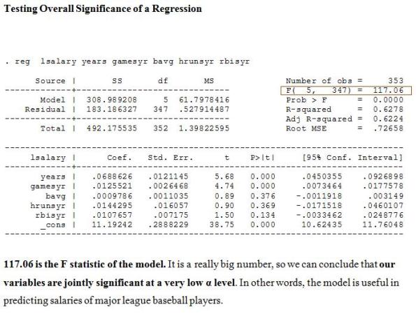
There is one special case of F-test that we want to test the overall significance of a model. In other words, we want to know if the regression model is useful at all, or we would need to throw it out and consider other variables. This is rarely the case, though.

~~~~~~~~~~~000~~~~~~~~~~~

This was such a painful and lengthy post. It has so many formulas that I had to do it in Microsoft Words and then convert it into several pictures…. I hope I made sense, though. =)

Let’s just keep in mind that the F test is for joint significance. That means we want to see whether or not a group of variables should be kept in the model.

Also, unlike the t distribution (bell shaped curve), F distribution is skewed to the right, with the smallest value is 0. Therefore, we would reject the null hypothesis if F-statistic (from the formula) is greater than critical-F (from the F table).

Single Linear Combinations of Parameters

Single Linear Combinations of Parameters means we are to test the linear relationship between two parameters in our multiple regression analysis. The simplest case can be

H₀: β₁ = β₂

Or H₀:  β₁ = 10β₂

Our hypothesis can be pretty much anything, as long as β₁ and β₂ has linear relationship.

Note that we are to test whether or not the effects of the two x variables on y have a linear relationship, NOT the linear relationship between the two x variables on each other (that is the case of perfect multicollinearity).

For example, we are interested in testing

H₀: β₁ = β₂

H₁: β₁ ≠ β₂

FIRST METHOD

Set θ = β₁ – β₂, then we will have

H₀: θ = 0
H₁: θ ≠ 0

–Set α (if not given, assume it to be .05)

–Find critical value: df=n-k-1 (k is the number of x variables), then use the t-table to find critical value.

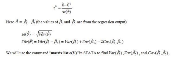
–Calculate test statistic:

(That output above was an example from my class notes.)

Therefore,

–Decision: to reject H₀ or not (by comparing t⁰ _­ with the critical value)

–Conclusion:

If we reject H₀ (β₁ = β₂), we will conclude that β₁ is statistically different from β₂ at α level.

If we fail to reject H₀ (β₁ = β₂), we will conclude that β₁ is not statistically different from β₂ at α level.

=========

Crazy enough, huh? There is another method that may look easier:

SECOND METHOD

-Set θ = β₁ – β₂, then β₁ = θ + β₂

-Substitute β₁ in our original model by θ + β₂

y= β₀ + β₁x₁ +  β₂x₂ +  β₃x₃ + u

y= β₀ + (θ + β₂)x₁+  β₂x₂ +  β₃x₃ + u  = β₀ + θx₁+  β₂(x₁+x₂) + β₃x₃ + u

Now our 3 variables in the model are x_1, x₁+x_2, x₃

-Construct a new variable that is the sum of x₁ and x₂ (in STATA) by using the command

gen totx12 =  x₁ + x₂

_{“totx12” is just the name of the new variable.}

-Run the regression of y on x₁, totx12, and x₃

-Test:

H₀: θ = 0
H₁: θ ≠ 0

Now we can look at the t-ratio or p-value of the coefficient on x₁ (coefficient on x₁ is now θ) then make our decision whether or not to reject H₀.